Plotting CellPhoneDB results

2024-04-19

ktplots

Welcome to ktplots! This is a R package to help visualise CellPhoneDB results. Here, we will go through a quick tutorial on how to use the functions in this package.

For a python port of ktplots, please check out my other repository.

Installation instructions

You can install the package via devtools::install_github() function in R

if (!requireNamespace("devtools", quietly = TRUE)) {
    install.packages("devtools")
}
if (!requireNamespace("BiocManager", quietly = TRUE)) {
    install.packages("BiocManager")
}
devtools::install_github("zktuong/ktplots", dependencies = TRUE)

Usage instructions

library(ktplots)

There is a test dataset in SingleCellExperiment format to test the functions.

library(SingleCellExperiment)
data(kidneyimmune)
# Some functions accept Seurat objects too.

The data is downsampled from the kidney cell atlas.

For more info, please see Stewart et al. kidney single cell data set published in Science 2019.

Prepare input

We will need 3 files to use this package, a SingleCellExperiment (or Seurat; some functions only accepts the former) object that correspond to the object you used for CellPhoneDB and the means.txt and pvalues.txt output. If you are using results from CellPhoneDB deg_analysis mode from version >= 3, the pvalues.txt is relevant_interactions.txt and also add degs_analysis = TRUE into all the functions below. deconvoluted is only used for plot_cpdb2/3/4.

# pvals <- read.delim("pvalues.txt", check.names = FALSE)
# means <- read.delim("means.txt", check.names = FALSE)
# decon = pd.read_csv("deconvoluted.txt", sep="\t")

# I've provided an example datasets
data(cpdb_output_stat) # ran with CellPhoneDB statistical analysis mode
data(cpdb_output_degs) # ran with CellPhoneDB degs analysis mode

Heatmap

The original heatmap plot from CellPhoneDB can be achieved with this reimplemented function.

plot_cpdb_heatmap(pvals = pvals_stat, cellheight = 10, cellwidth = 10)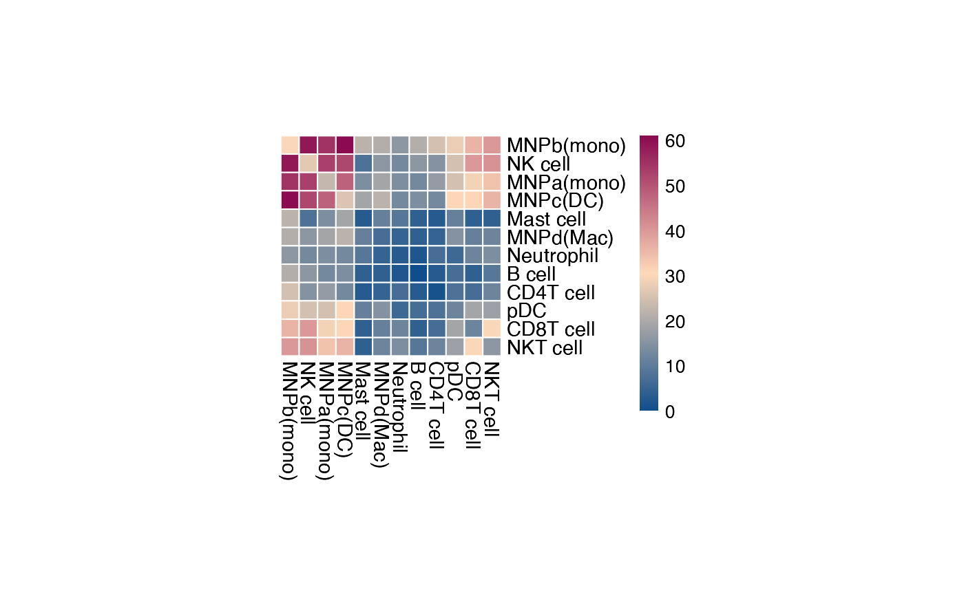

plot_cpdb_heatmap(pvals = rel_int_degs, cellheight = 10, cellwidth = 10, degs_analysis = TRUE)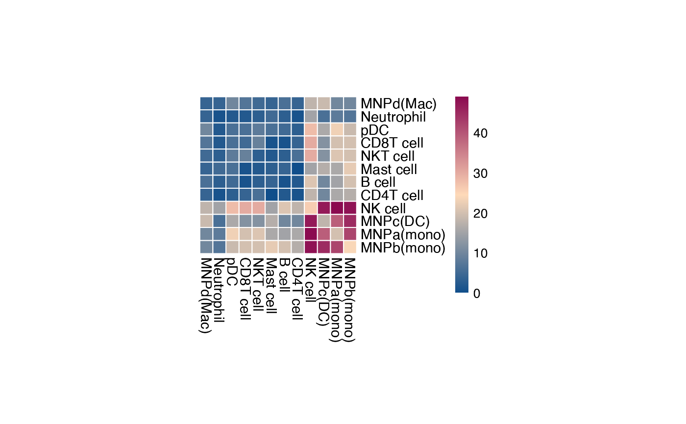

You can also specify specific celltypes to plot.

plot_cpdb_heatmap(pvals=pvals_stat, cell_types=c("NK cell", "pDC", "B cell", "CD8T cell"), cellheight = 10, cellwidth = 10)

The current heatmap is directional (check count_network and interaction_edges for more details in return_tables = True).

To obtain the heatmap where the interaction counts are not symmetrical, do:

plot_cpdb_heatmap(pvals = pvals_stat, cellheight = 10, cellwidth = 10, symmetrical = FALSE)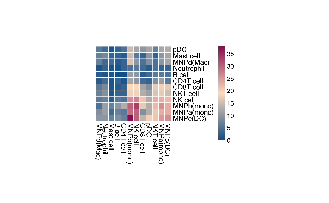

The values for the symmetrical=FALSE mode follow the direction of the L-R direction where it’s always moleculeA:celltypeA -> moleculeB:celltypeB.

Therefore, if you trace on the x-axis for celltype A [MNPa(mono)] to celltype B [CD8T cell] on the y-axis:

A -> B is 18 interactions

Whereas if you trace on the y-axis for celltype A [MNPa(mono)] to celltype B [CD8T cell] on the x-axis:

A -> B is 9 interactions

symmetrical=TRUE mode will return 18+9 = 27

Dot plot

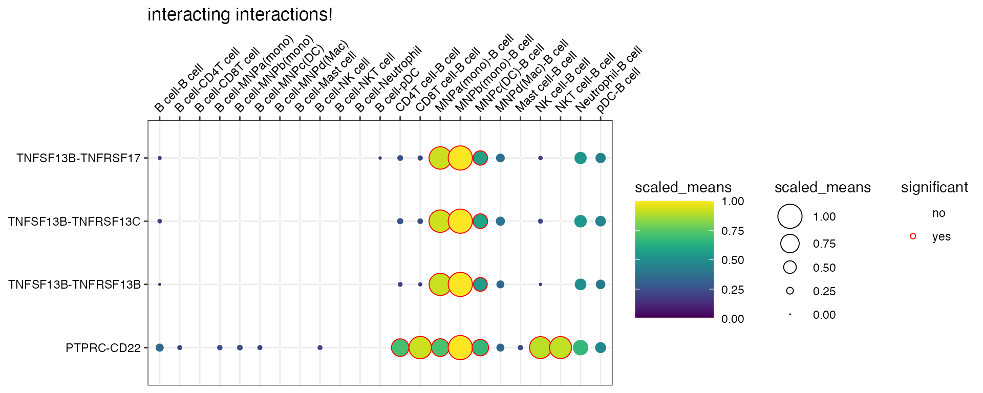
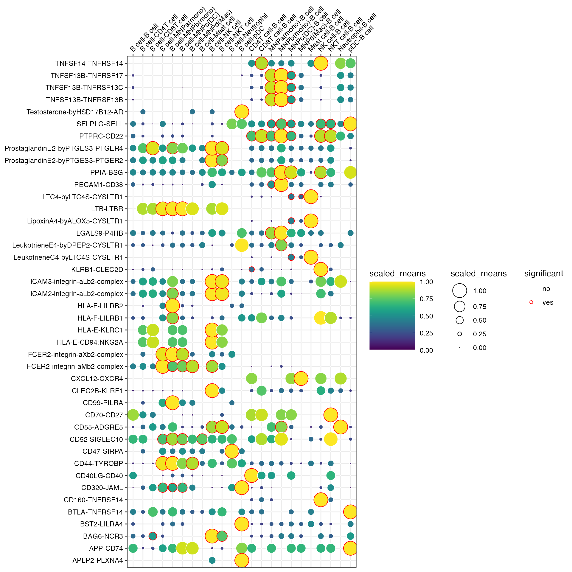
plot_cpdb

A simple usage of plot_cpdb is as follows:

plot_cpdb(
    scdata=kidneyimmune,
    cell_type1="B cell",
    cell_type2=".",  # this means all cell-types
    celltype_key="celltype",
    means=means_stat,
    pvals=pvals_stat,
    genes=c("PTPRC", "TNFSF13"),
    title="interacting interactions!",
)

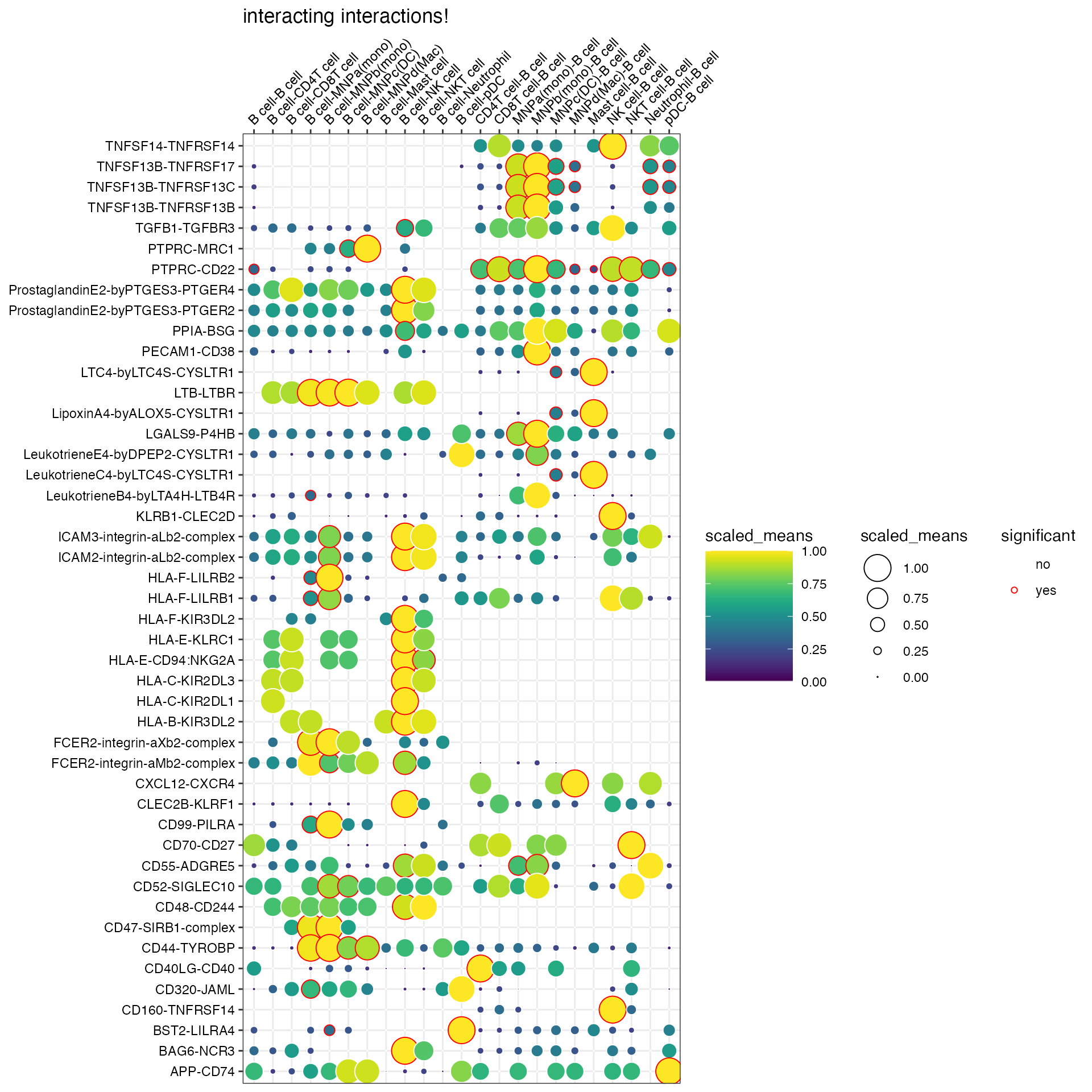
You can keep the original id_cp_interaction value in the name too.

plot_cpdb(
    scdata=kidneyimmune,
    cell_type1="B cell",
    cell_type2=".",  # this means all cell-types
    celltype_key="celltype",
    means=means_stat,
    pvals=pvals_stat,
    genes=c("PTPRC", "TNFSF13"),
    title="interacting interactions!",
    keep_id_cp_interaction=TRUE,
)

plot_cpdb(
    scdata=kidneyimmune,
    cell_type1="B cell",
    cell_type2=".",  # this means all cell-types
    celltype_key="celltype",
    means=means_degs,
    pvals=rel_int_degs,
    degs_analysis=TRUE,
    genes=c("PTPRC", "TNFSF13"),
    title="interacting interactions!",
)

Or don’t specify either and it will try to plot all significant interactions.

plot_cpdb(
    scdata=kidneyimmune,
    cell_type1="B cell",
    cell_type2=".",
    celltype_key="celltype",
    means=means_stat,
    pvals=pvals_stat,
)

plot_cpdb(
    scdata=kidneyimmune,
    cell_type1="B cell",
    cell_type2=".",  # this means all cell-types
    celltype_key="celltype",
    means=means_degs,
    pvals=rel_int_degs,
    degs_analysis=TRUE,
    title="interacting interactions!",
)

You can also try an alternative visualisation inspired by how squidpy displays the results:

plot_cpdb(
    scdata=kidneyimmune,
    cell_type1="B cell",
    cell_type2=".",
    celltype_key="celltype",
    means=means_stat,
    pvals=pvals_stat,
    genes=c("PTPRC", "CD40", "CLEC2D"),
    default_style=FALSE
)

you can also toggle options to splitby_key and gene_family:

data(cpdb_output) # this is a different dataset where the "Experiment" was appended to the "celltype" 

plot_cpdb(
    scdata = kidneyimmune,
    cell_type1 = "B cell",
    cell_type2 = "Neutrophil|MNPc|NK cell",
    celltype_key = "celltype",
    means = means,
    pvals = pvals,
    splitby_key = "Experiment",
    gene_family = "chemokines"
)

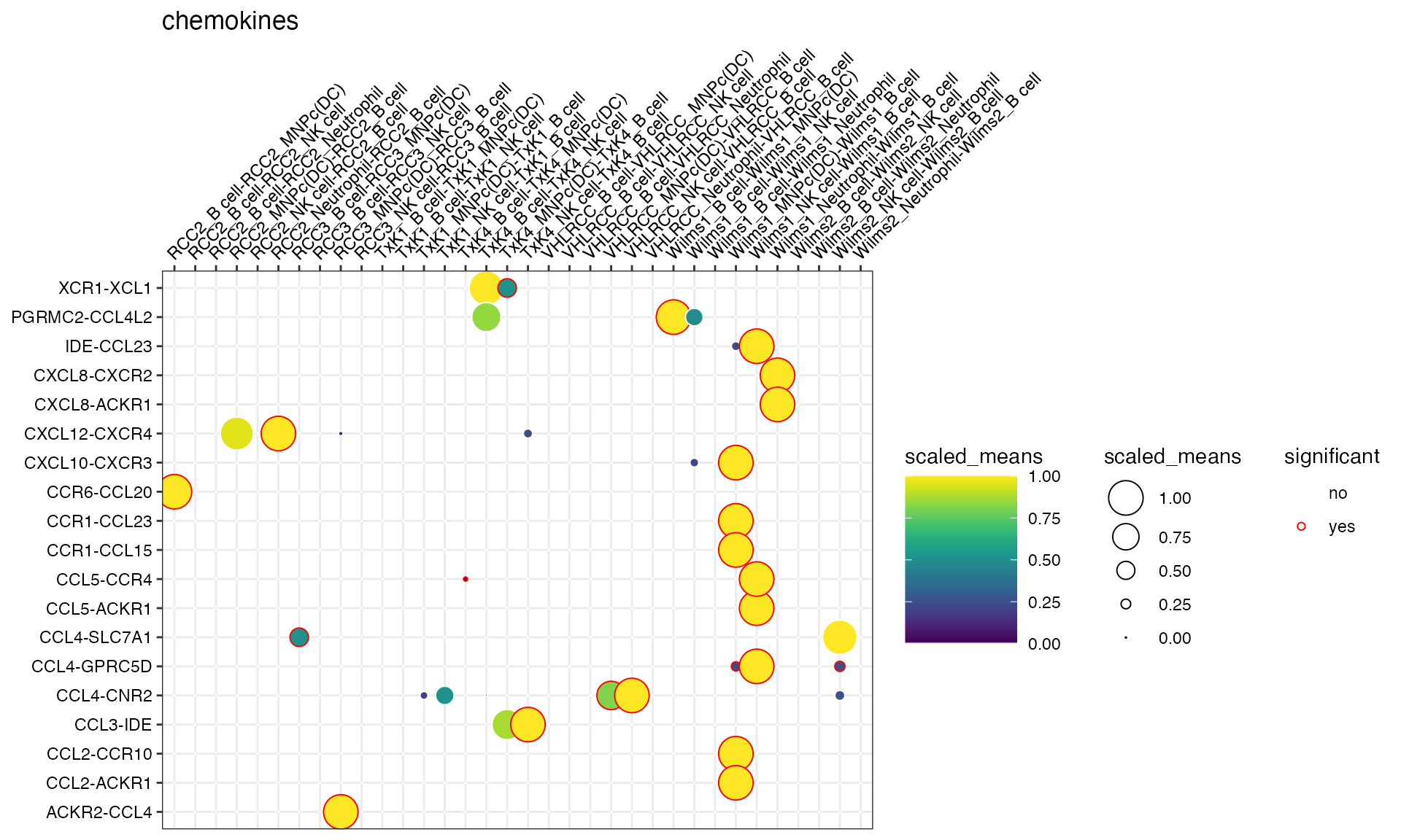
if genes and gene_family are both not specified, the function will try to plot everything.

Specifying keep_significant_only will only keep those that are p<0.05.

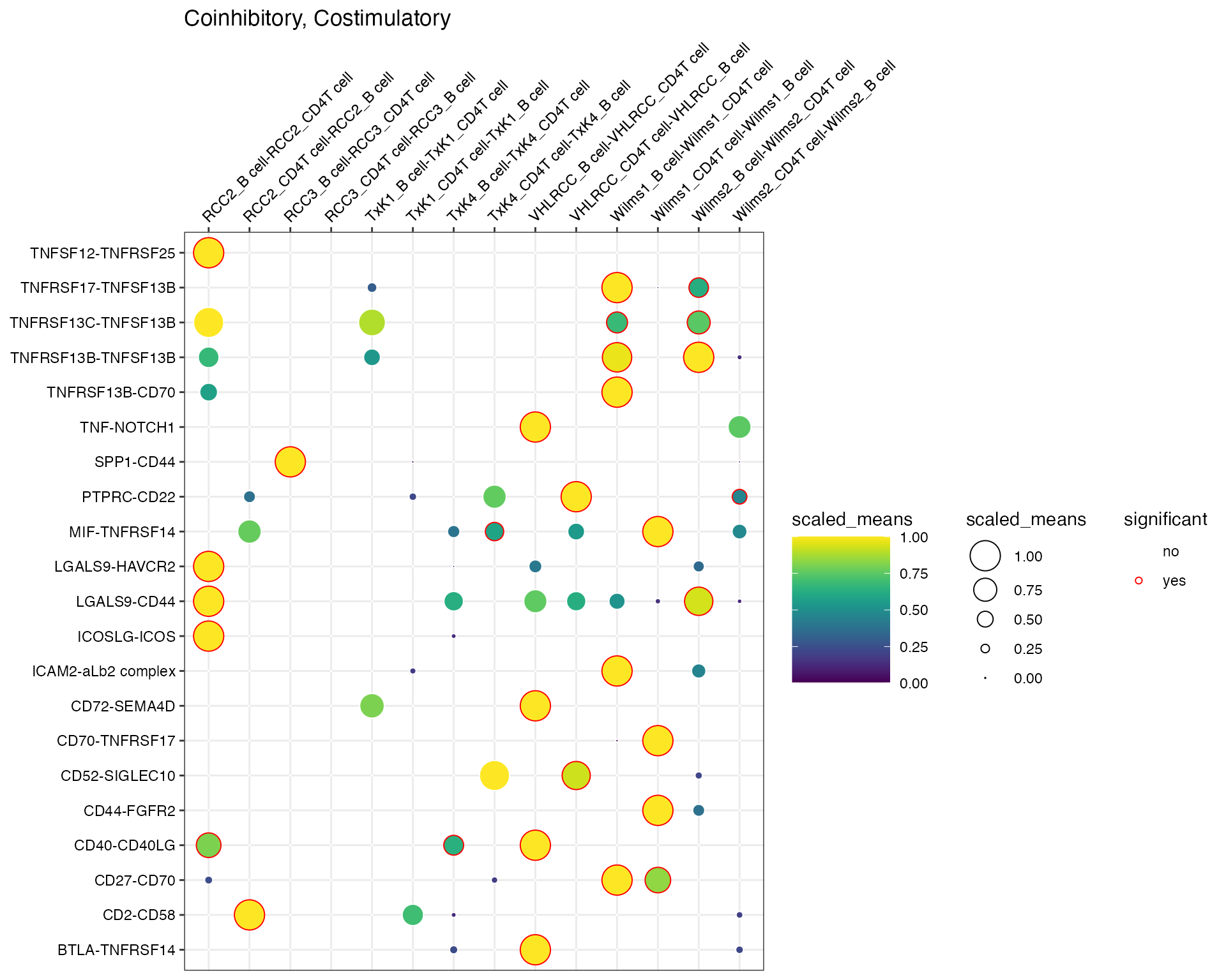
You can also specify more than 1 gene families:

plot_cpdb(
    scdata = kidneyimmune,
    cell_type1 = "B cell",
    cell_type2 = "CD4T cell",
    celltype_key = "celltype",
    means = means,
    pvals = pvals,
    splitby_key = "Experiment",
    gene_family = c("Coinhibitory", "Costimulatory"),
    cluster_rows = FALSE # ensures that the families are separate,
)

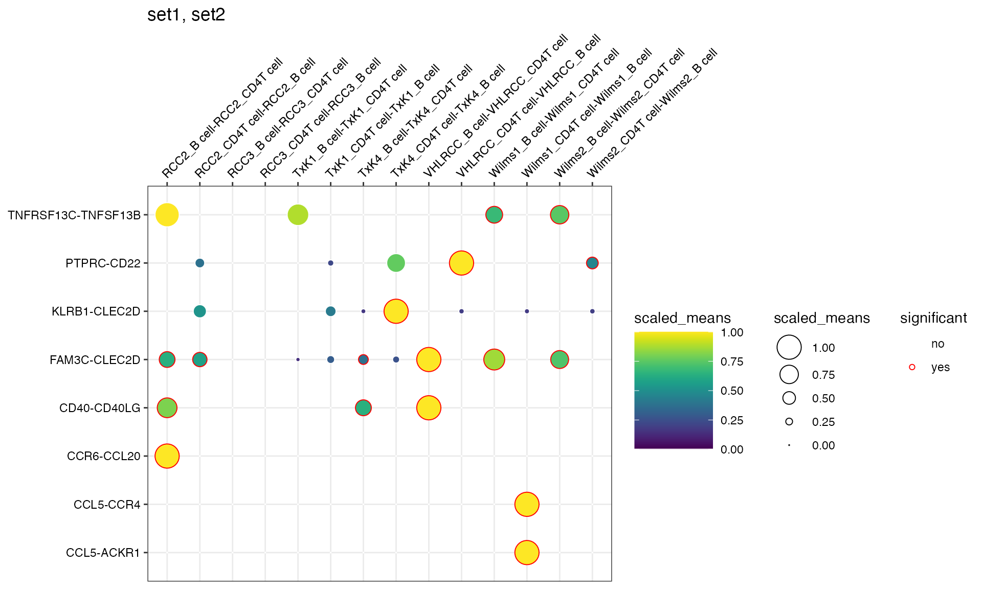
And also provide custom families as a data.frame.

df <- data.frame(set1 = c("CCR6", "CCL20", "CXCL10", "CCR3", "TNFRSF13C"), set2 = c("CCL5", "CCR4", "PTPRC", "CD40", "CLEC2D"))
plot_cpdb(
    scdata=kidneyimmune,
    cell_type1 = "B cell",
    cell_type2 = "CD4T cell",
    celltype_key = "celltype",
    means = means,
    pvals = pvals,
    splitby_key = "Experiment",
    gene_family = c("set1", "set2"),
    custom_gene_family = df,
)

combine_cpdb

For the splitby_key option to work, the annotation in the meta file must be defined in the following format:

{splitby_key}_{celltype_key}

so to set up an example vector, it would be something like:

annotation <- paste0(kidneyimmune$Experiment, "_", kidneyimmune$celltype)

The recommended way to use splitby_key is to prepare the data with combine_cpdb like in this example:

# Assume you have 2 cellphonedb runs, one where it's just naive and the other is treated, you will end up with 2 cellphonedb out folders
# remember, the celltype labels you provide to cellphonedb's meta.txt should already be like {splitby_key}_{celltype_key}
# so the two meta.txt should look like:

# naive file
# ATTAGTCGATCGTAGT-1    naive_CD4Tcell
# ATTAGTGGATCGTAGT-1    naive_CD4Tcell
# ATTAGTCGACCGTAGT-1    naive_CD8Tcell
# ATTAGTCGATCGTAGT-1    naive_CD8Tcell
# ATGAGTCGATCGTAGT-1    naive_Bcell
# ATTAGTCGATCGTGGT-1    naive_Bcell

# treated file
# ATTAGTCAATCGTAGT-1    treated_CD4Tcell
# ATTAGTGGATCGTAGT-1    treated_CD4Tcell
# ATTAGTCGACCATAGT-1    treated_CD8Tcell
# ATTAGTAGATCGTAGT-1    treated_CD8Tcell
# ATGAGTCGATCGTAAT-1    treated_Bcell
# ATTAGTCGATCGTGAT-1    treated_Bcell

# one you have set that up correctly, you can then read in the files.
naive_means <- read.delim("naive_out/means.txt", check.names = FALSE)
naive_pvals <- read.delim("naive_out/pvalues.txt", check.names = FALSE)
naive_decon <- read.delim("naive_out/deconvoluted.txt", check.names = FALSE)

treated_means <- read.delim("treated_out/means.txt", check.names = FALSE)
treated_pvals <- read.delim("treated_out/pvalues.txt", check.names = FALSE)
treated_decon <- read.delim("treated_out/deconvoluted.txt", check.names = FALSE)

means <- combine_cpdb(naive_means, treated_means)
pvals <- combine_cpdb(naive_pvals, treated_pvals)
decon <- combine_cpdb(naive_decon, treated_decon)

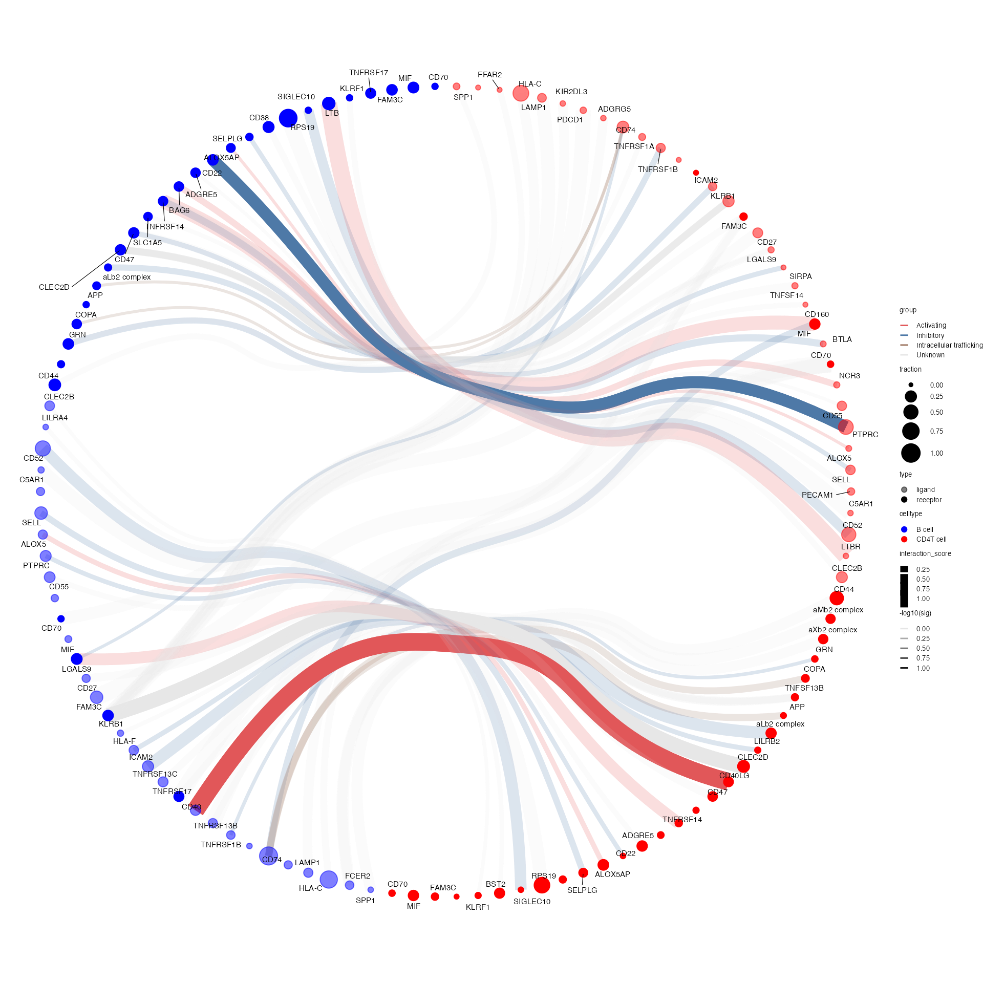
plot_cpdb(...)

plot_cpdb2

Generates a circos-style wire/arc/chord plot for cellphonedb results.

This function piggy-backs on the original plot_cpdb function and generates the results like this:

Please help contribute to the interaction grouping list here!

Credits to Ben Stewart for coming up with the base code!

data(cpdb_output2) # legacy reasons
plot_cpdb2(
    scdata = kidneyimmune,
    cell_type1 = "B cell",
    cell_type2 = ".",
    celltype_key = "celltype", # column name where the cell ids are located in the metadata
    means = means2,
    pvals = pvals2,
    deconvoluted = decon2, # new options from here on specific to plot_cpdb2
    desiredInteractions = list(
        c("CD4T cell", "B cell"),
        c("B cell", "CD4T cell")
    ),
    interaction_grouping = interaction_annotation,
    edge_group_colors = c(
        "Activating" = "#e15759",
        "Chemotaxis" = "#59a14f",
        "Inhibitory" = "#4e79a7",
        "Intracellular trafficking" = "#9c755f",
        "DC_development" = "#B07aa1",
        "Unknown" = "#e7e7e7"
    ),
    node_group_colors = c(
        "CD4T cell" = "red",
        "B cell" = "blue"
    ),
)

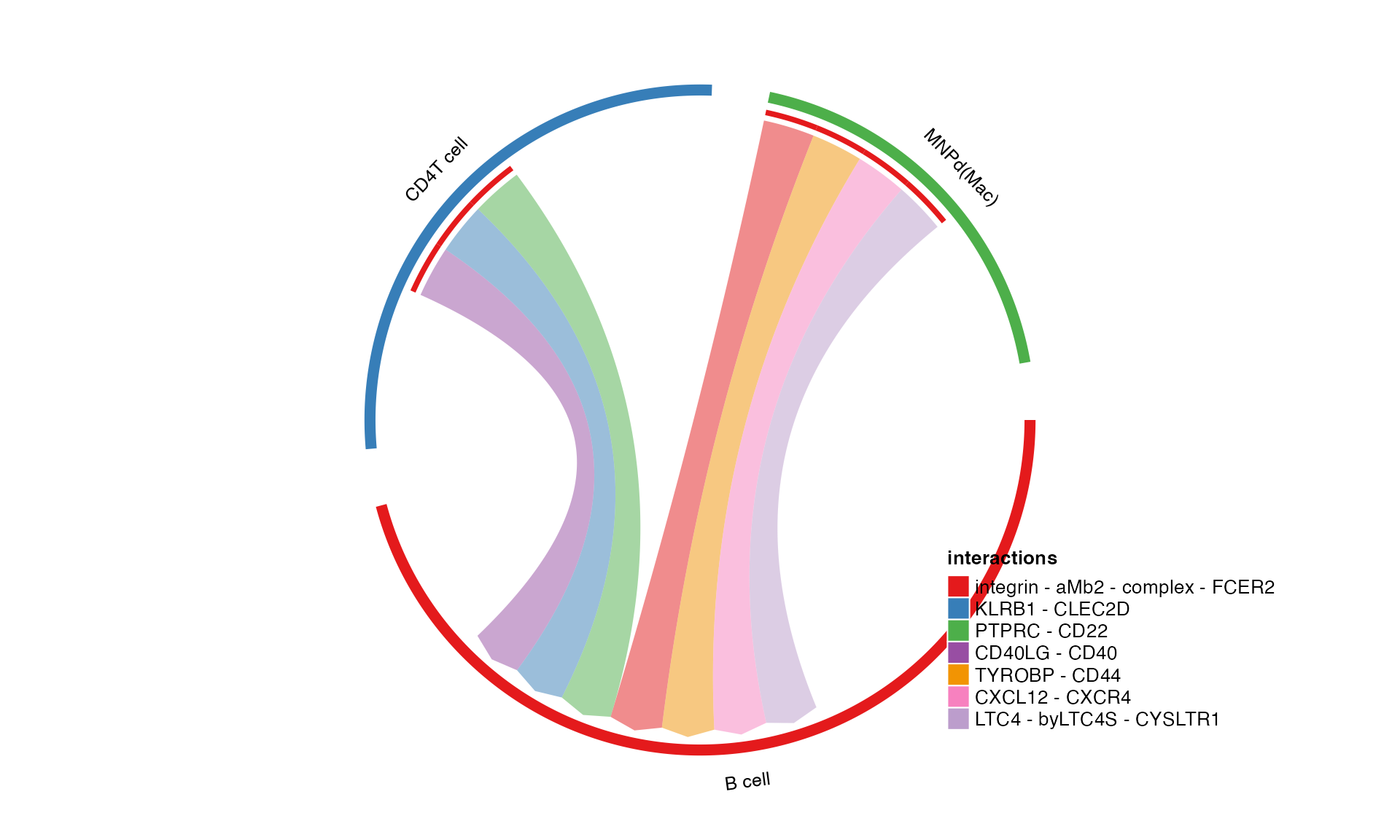
plot_cpdb3

Generates a chord diagram inspired from CellChat’s way of showing the data!

Usage is similar to plot_cpdb2 but with reduced options. Additional kwargs are passed to plot_cpdb.

plot_cpdb3(
    scdata = kidneyimmune,
    cell_type1 = "B cell",
    cell_type2 = "CD4T cell|MNPd",
    celltype_key = "celltype", # column name where the cell ids are located in the metadata
    means = means_stat,
    pvals = pvals_stat,
    deconvoluted = decon_stat # new options from here on specific to plot_cpdb3
)

plot_cpdb4

New! Alternate way of showing the chord diagram for specific interactions!

Usage is similar to plot_cpdb3 but with additional required interaction option. Additional kwargs are passed to plot_cpdb.

plot_cpdb4(
    scdata = kidneyimmune,
    interaction = "CLEC2D-KLRB1",
    cell_type1 = "NK",
    cell_type2 = "Mast",
    celltype_key = "celltype",
    means = means_stat,
    pvals = pvals_stat,
    deconvoluted = decon_stat
)

or specify more than 1 interactions + only show specific cell-type type interactions!

plot_cpdb4(
    interaction = c("CLEC2D-KLRB1", "CD40-CD40LG"),
    cell_type1 = "NK|B", cell_type2 = "Mast|CD4T",
    scdata = kidneyimmune,
    celltype_key = "celltype",
    means = means2,
    pvals = pvals2,
    deconvoluted = decon2,
    desiredInteractions = list(
        c("NK cell", "Mast cell"),
        c("NK cell", "NKT cell"),
        c("NKT cell", "Mast cell"),
        c("B cell", "CD4T cell")
    ),
    keep_significant_only = TRUE,
)

Other useful functions

geneDotPlot

Plotting gene expression dot plots heatmaps.

library(ggplot2)
# Note, this conflicts with tidyr devel version
geneDotPlot(
    scdata = kidneyimmune, # object
    genes = c("CD68", "CD80", "CD86", "CD74", "CD2", "CD5"), # genes to plot
    celltype_key = "celltype", # column name in meta data that holds the cell-cluster ID/assignment
    splitby_key = "Project", # column name in the meta data that you want to split the plotting by. If not provided, it will just plot according to celltype_key
    standard_scale = TRUE
) + theme(strip.text.x = element_text(angle = 0, hjust = 0, size = 7)) + small_guide() + small_legend()
#> data provided is a SingleCellExperiment/SummarizedExperiment object
#> extracting expression matrix
#> attempting to subset the expression matrix to the 6 genes provided
#> found 6 genes in the expression matrix
#> preparing the final dataframe ...
#> setting minimum percentage of cells expressing gene to be 5% of cluster/cell-type
#> the following genes are removed
#> NULL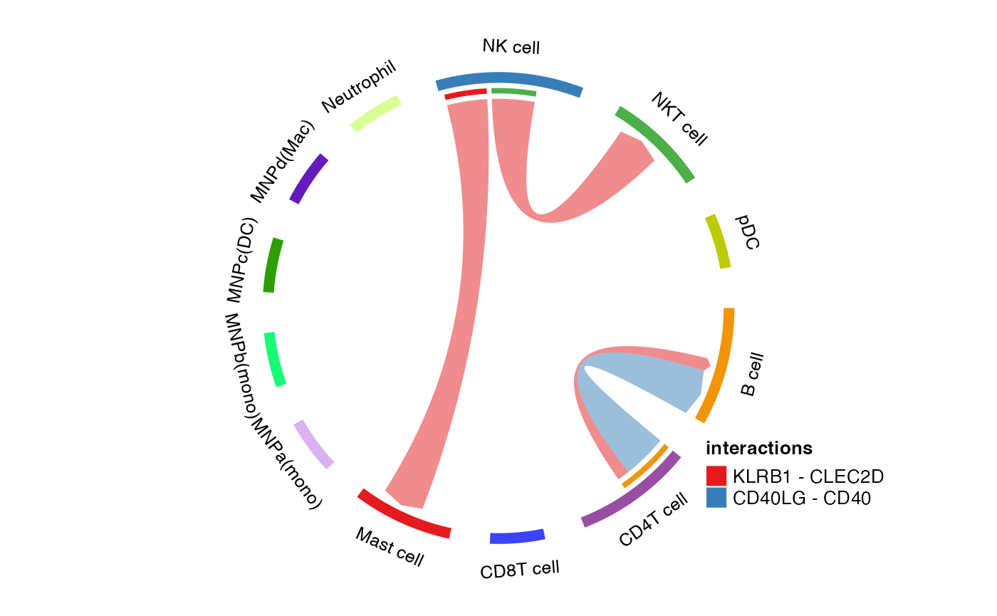

Citation

If you find these functions useful, please consider leaving a star and cite this preprint:

Troulé K, Petryszak R, Prete M, Cranley J, Harasty A, Tuong ZK, Teichmann SA, Garcia-Alonso L, Vento-Tormo R. CellPhoneDB v5: inferring cell-cell communication from single-cell multiomics data. arXiv preprint arXiv:2311.04567. 2023 Nov 8.

Thank you!